How We Made Sense of Thousands of Keywords

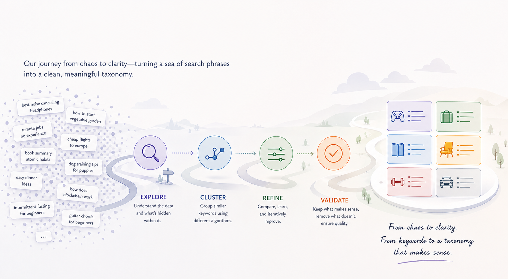
Imagine being handed five thousand search phrases someone might type into Google about skincare — face wash for men, vitamin c serum, sunscreen for dry skin, kid's body lotion, and so on — and being asked to sort them into a small number of meaningful groups. That's the problem we're trying to solve, automatically, for every customer we onboard.

The first time we built this, the output was a mess. On a recent skincare-domain test run with 5,874 keywords, our pipeline produced 1,189 groups. After an LLM clean-up pass, we ended up with 14 — but the silhouette score was 0.107, which essentially means the groups weren't meaningfully different from each other. Random would score about the same.

This post is the story of how we got from there to a partition that actually compresses the universe into a clean taxonomy — by walking through four different clustering algorithms and learning something specific from each.

A quick reference

We'll mention these terms throughout:

k-means — A clustering algorithm where you specify the number of groups (k) up front, and it finds k cluster centers and assigns each point to the nearest one.
HDBSCAN — A clustering algorithm that finds groups by looking for dense regions of points. Sparse points get labelled as "noise."
Leader algorithm — A simple, fast clustering pass: walk through your data once, and either add each new point to the nearest existing group (if it's close enough) or start a brand new group.
Leiden algorithm — A graph-based community detection algorithm. You build a graph of "who is similar to whom," and Leiden finds groups where the connections inside a group are much denser than the connections between groups.
Modularity — A score from –1 to 1 that measures how well a partition splits a graph into communities. Higher means the connections inside groups are unusually dense compared to what you'd expect by chance. Above 0.3 is meaningful structure; above 0.5 is strong.
Constant Potts Model (CPM) — An alternative scoring rule for Leiden that fixes a known weakness of standard modularity (it tends to swallow small dense communities into bigger ones) and gives you a single resolution knob to control how fine-grained the groups should be.

With that out of the way — here's how we got from one algorithm to the other.

Stop one: k-means

What it does

You tell k-means in advance how many groups to make — that's the k. It places k cluster centers in the embedding space, assigns every keyword to the nearest center using cosine similarity, and iteratively moves the centers around until each one sits at the centroid of its assigned points.

What we tried

Nothing — and that was a deliberate decision.

What we got

For us, the value of clustering is discovering the structure of a customer's keyword universe. We don't know in advance whether a given domain has 12 distinct intent groups or 80, and any number we picked up front would be wrong for half the customers we onboard.

There are heuristics for choosing k after the fact (the elbow method, silhouette sweeps), but those all reduce to running k-means many times and post-hoc justifying a number. That's not discovery; it's a parameter we'd have to defend, customer by customer. We needed cluster count to come from the data itself.

So we skipped k-means and looked for an algorithm that figures out the number of groups on its own.

Stop two: HDBSCAN

What it does

HDBSCAN looks for dense regions of points. The intuition is that real clusters are places where points crowd together; the empty space between clusters is sparse. So it scans the dataset, finds the dense pockets, calls them clusters, and labels everything in the sparse in-between as "noise."

This is appealing because the algorithm doesn't ask you how many clusters to find. It tells you, based on where the density actually is.

What we tried

We ran HDBSCAN on a real production snapshot from a different domain — an e-signature SaaS keyword universe — and compared it side-by-side with our existing Leader pipeline:

Algorithm	Configuration	Result
Leader + threshold merge	assign_threshold=0.72, merge_threshold=0.80	48 main clusters + 129 long-tail
HDBSCAN	min_cluster_size=3, min_samples=2	2 clusters + 3 noise points

What we got

HDBSCAN collapsed almost the entire universe into a single giant cluster of 2,443 keywords (top terms: esign, e-sign, electronic signature, electronic signature pdf), with a tiny secondary cluster and 3 stray points labelled as noise. Tweaking min_cluster_size and min_samples either produced the same blob or fragmented things into pure noise.

This is a known HDBSCAN behaviour in high-dimensional embedding spaces. HDBSCAN looks for variable density. But in a 1,536-dimensional space where related keywords sit at near-uniform cosine distances from each other, density is roughly the same everywhere. Either everything looks like one dense region or nothing does. There's no gradient for HDBSCAN to draw boundaries from.

We could have spent more time tuning, or stacked UMAP on top to manufacture artificial density variation, but the failure mode felt structural. We needed something that didn't depend on density gradients at all.

Stop three: the Leader algorithm

What it does

Leader is the simplest clustering algorithm you can imagine. Walk through your keywords in some order. For each one:

If its embedding is similar enough to the centroid of an existing cluster (above the assign threshold), drop it into that cluster and update the centroid.
Otherwise, start a brand new cluster with this keyword as the first member.

That's it. One pass through the data, no iteration. After Leader runs, an LLM gives every cluster a short human-readable label based on its top keywords. A second LLM pass then looks at the cluster labels and merges any that describe the same intent.

What we tried

We built the full Leader pipeline. We tuned the assign threshold to 0.72 and the merge threshold to 0.80, then handed the labelled clusters to an LLM to consolidate any with shared intent.

What we got

On a 5,874-keyword skincare universe, the pipeline produced 1,189 clusters.

The core problem was structural: Leader has no global view. The first keyword to arrive in a region anchors a bucket, and every later keyword's fate depends on whether its cosine similarity to that bucket's centroid happens to clear the assign threshold. A keyword that misses by a hair starts its own bucket, even if a slightly different processing order would have placed both in the same group. Run the same data with a different sort order, and you get a different partition.

That order-dependence and locality is what produced the fragmentation. We needed an algorithm that looks at the whole picture before deciding.

Stop four: discovering Graphify

We were stuck. Density-based clustering had collapsed. Threshold-tuning Leader was a dead end.

Around this time, Graphify crossed our radar — an open-source project that turns a codebase into a queryable knowledge graph. It uses Tree-sitter for code parsing, NetworkX for graph storage, and Leiden community detection for grouping related code entities into navigable clusters that become nodes in a higher-level graph.

What grabbed our attention wasn't the codebase parsing — it was the architecture. Graphify wasn't doing keyword clustering, but it was solving a structurally similar problem: take a large set of related entities, build a graph from their relationships, and use community detection to find the natural groupings. The clusters then become the nodes in a higher-level graph.

That's exactly the shape of our problem. We wanted keyword clusters that could later become the nodes of topic and intent maps. The recipe transferred.

So we read the algorithm choice carefully and went down the Leiden rabbit hole.

Stop five: Leiden community detection

What it does

Leiden takes a completely different approach. Instead of looking at keywords as points in space and asking "which centroid is closest," it looks at them as nodes in a graph and asks "which nodes are most densely connected to each other?"

Step by step:

Build a graph. Each keyword is a node. Draw edges between keywords whose embeddings are similar — the more similar, the heavier the edge. (We used cosine similarity for the edge weight, with a floor of 0.55 to filter out weak connections.)
Find communities. Leiden looks for groups of nodes where the connections within the group are much denser than the connections between groups. That density imbalance is exactly what modularity measures — and Leiden's job is to find the partition that maximizes it.
Refine. Leiden adds a refinement phase that guarantees every community is internally well-connected (no broken-off pieces hiding in the same group).

The key shift: there are no thresholds for cluster boundaries. Leiden looks at the whole graph, sees where the natural seams are, and partitions there. Cluster count emerges from the data, not from a parameter.

<text x="115" y="60" text-anchor="middle" class="nlabel" font-weight="600" fill="#2563eb">face wash / cleansers</text> <text x="410" y="60" text-anchor="middle" class="nlabel" font-weight="600" fill="#ea580c">sunscreen / SPF</text> <text x="270" y="270" text-anchor="middle" class="nlabel" font-weight="600" fill="#059669">moisturizer / lotion</text>

<g transform="translate(20,255)"> <line x1="0" y1="6" x2="30" y2="6" class="edge-strong"/> <text x="38" y="10" class="label">strong similarity</text> <line x1="160" y1="6" x2="190" y2="6" class="edge-weak"/> <text x="198" y="10" class="label">weak/cross-community</text> </g> </svg>

This is also where the Constant Potts Model (CPM) comes in. Standard modularity has a known weakness — it tends to absorb small but genuinely distinct communities into bigger ones (the so-called resolution limit). CPM scores the same partition slightly differently and gives you a cleaner resolution knob: turn it up to break things into smaller, more specific groups; turn it down for fewer, broader groups. We used CPM throughout.

What we tried

We built a small Python lab next to our backend (the gold-standard implementations of Leiden — leidenalg and python-igraph — are Python-only) and ran the algorithm on real production data. Specifically, we dumped a recent skincare-domain run from Redis, re-embedded the 5,837 unique keywords with text-embedding-3-small, and swept through combinations of two parameters:

Edge threshold — how strict to be about which keyword pairs even get an edge in the graph (we tried 0.45 to 0.60).
Resolution — how fine-grained the communities should be (we tried 0.05 to 0.70).

We also tried two staging approaches: feeding Leiden the existing 1,189 Leader cluster centroids (treating it as a clean-up layer), and feeding it all 5,874 keywords directly (treating it as a full replacement).

What we got

The centroid-as-nodes experiment told us something useful about Leader:

edge threshold	resolution	communities	modularity	biggest community
0.45	0.05	67	0.285	602 Leader buckets (4,545 keywords)
0.45	0.15	98	0.396	190 buckets
0.45	0.30	134	0.318	136 buckets

At low resolution, Leiden pulled 602 of the 1,189 Leader buckets — 77% of the universe — into a single mega-community. That looked like a failure but was actually a diagnostic: Leiden was correctly identifying connectivity that Leader had failed to consolidate. The 1,189 buckets were heavily over-fragmented; many "different" buckets were the same intent broken into pieces.

The lesson: don't use Leiden as a clean-up pass. Replace Leader entirely.

So we ran the keywords-as-nodes experiment:

edge threshold	resolution	communities	modularity	biggest community
0.45	0.15	122	0.437	1,003 keywords
0.50	0.15	185	0.563	783 keywords
0.55	0.15	322	0.593	699 keywords
0.55	0.30	432	0.491	606 keywords
0.60	0.15	477	0.579	574 keywords

The best modularity landed at edge threshold 0.55 and resolution 0.15: 322 communities, modularity 0.593. Anything above 0.5 indicates strong community structure, so this is a solid score for real-world data.

But the headline isn't 322. It's what the top communities actually contain:

#	size	top theme
0	699	scrubs / exfoliators
1	662	face wash / cleansers
2	615	sunscreen / SPF
3	514	body lotion / moisturizer
4	360	face masks / sheet masks
5	299	face moisturizers (separate from body)
6	240	eye drops (off-domain)
7	186	face serums (generic)
8	184	vitamin C serums

This is what a real keyword taxonomy looks like. Seven broad product categories, plus mid-level subcategories like "vitamin C serums" cleanly separated from "face serums" — a split the Leader pipeline never made.

The off-domain "eye drops" community surfaced as its own group — exactly right. That's a downstream filtering decision, not a clustering one. The point is that the structure was visible, separately, in the partition.

What we learned

A few things stood out, and they generalize beyond keyword clustering.

Cluster count should come from the data, not from a parameter

This was the lens that ruled out k-means before we ever ran it, and it's the same lens that made HDBSCAN attractive on paper and Leiden attractive in practice. Across the customer domains we onboard, the right cluster count varies enormously — picking a number up front and tuning everything else to fit it is the wrong shape of problem.

Density-based clustering breaks down in dense embedding spaces

HDBSCAN works beautifully when your data has variable density — clear high-density clumps separated by sparse regions. Modern embedding spaces don't look like that. Related items sit at near-uniform distances, density gradients vanish, and HDBSCAN either sees one giant blob or no clusters at all. This isn't a tuning issue; it's a structural mismatch.

Local, order-dependent passes fragment in dense embedding spaces

Skincare is densely interconnected: "moisturizer" sits near "face cream" sits near "lotion" sits near "body butter." In that kind of space, an algorithm that decides each keyword's home one at a time, based on the order it arrives, will spread closely-related keywords across many small buckets. Modularity is the right tool because it asks a different question: given the connectivity of the whole graph, where are the natural seams?

Borrowing recipes from adjacent domains works

Graphify is a code-knowledge-graph tool, not a keyword research tool. We had no business reading their clustering code. But the underlying problem — group related entities, then make those groups the nodes of a higher-level graph — is identical to ours. Reading their algorithmic choices saved us from re-deriving the recipe ourselves.

The transferable lesson: when you're stuck on a clustering problem, look for projects in adjacent domains that have already solved a structurally similar version. The math often ports even when the data doesn't.

Where this leaves us

The lab confirms what we suspected when we saw the cluster count. Leiden on a properly-constructed graph produces a partition that is qualitatively better than anything the threshold-based pipeline produced — coherent broad categories, meaningful subcategorization, and an order-of-magnitude reduction in total cluster count without losing detail.

What's left:

Validating on a second domain. Skincare is densely connected; we want to confirm the recipe holds for, say, B2B SaaS or kids' apparel before locking it in.
Designing the production integration. The lab uses Python because leidenalg is the gold-standard implementation. Integrating into a NestJS backend means either porting to a Node Leiden library (quality varies) or running a Python sidecar. We'll likely take the sidecar route, fronted by a small HTTP service.
Bringing the LLM back in for what it's actually good at — labelling and final merge of a clean partition rather than triaging hundreds of fragmented buckets.

That last point is the thing that changed the most for us. Once the input is a well-formed, modularity-optimized partition, the LLM's role becomes much smaller and much more reliable: name the cluster, optionally combine two if they share intent. That's a problem it can solve.

The blog you're reading is mostly about an algorithm swap, but the actual lesson is about the division of labour. Embeddings define a similarity geometry. Graph algorithms find structure in that geometry. LLMs name the structure. We had been asking the LLM to do all three, and it was failing at the hardest one.

How We Made Sense of Thousands of Keywords

A quick reference

Stop one: k-means

What it does

What we tried

What we got

Stop two: HDBSCAN

What it does

What we tried

What we got

Stop three: the Leader algorithm

What it does

What we tried

What we got

Stop four: discovering Graphify

Stop five: Leiden community detection

What it does

What we tried

What we got

What we learned

Cluster count should come from the data, not from a parameter

Density-based clustering breaks down in dense embedding spaces

Local, order-dependent passes fragment in dense embedding spaces

Borrowing recipes from adjacent domains works

Where this leaves us

Is your brand visible in AI search?

Related Articles

Raven: Building a Trustworthy Inference Engine for Production LLM Systems

Beyond Dashboards: A Five-Layer Architecture for Proactive AI Search Visibility

How LLMs decide who to cite: The mechanics behind AI Search visibility